In general a signal can be approximated by a Fourier Series. In this blog I will represent the signal coming from the edges of the image containing my face using the Fourier representation.
Considering $t \in \mathcal{T} = [t_0, t_1] \subset \mathbb{R}$ be an input variable, $T = t_1 - t_0$ the length of the input domain, and $f(\cdot) : \mathcal{T} \rightarrow \mathbb{C}$ being the function that represents the edges signal in the 2D complex plane, the Fourier representation of the signal can be computed as:
Here $N$ is the number of components used for the approximating the input signal, the larger this number, the better the approximation. $T$ is the length of the input domain of $x$, $T = | \mathcal{T}| $.
Let's make an example by considering an image:
# Imports
import numpy as np
import matplotlib.pyplot as plt
from PIL import Image
from sklearn.cluster import KMeans
import cv2
import requests

# Load the image
url = 'https://guglielmocamporese.github.io/static/static/img/fourier/image.png'
image = np.array(Image.open(requests.get(url, stream=True).raw))
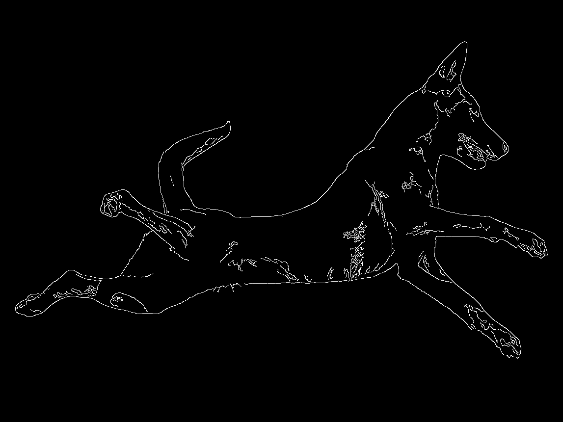
Now let's compute the edges of the image by low-pass filtering the image and using the Canny algorithm, already implemented in OpenCV.
# Compute the edges
def get_edges(x):
  """Extract edges from an image."""
  x = cv2.GaussianBlur(x, (5, 5), 0)
  x = cv2.Canny(x, 10, 200)
  return x

edges = get_edges(image)
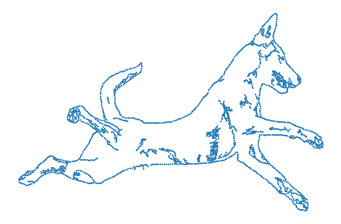
The next step is to reduce the number of points contained in the edges. To this end, I clustered these points reducing them from a number $\sim 13000$ to $n\_cluster=2000$ as follows:
The image above shows the cluster centers that fit the edges.
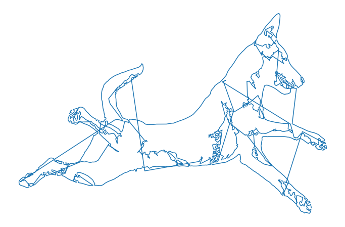
For now we have a set of points that builds up the edge signal, but this set is un-ordered since each point does not have the meaning of "neighbors". In the image below you can see this fact by connecting adjacent points in the set.
In order to solve the order issue, I designed a sorting algorithm that returns a set of ordered points using the euclidian distance.
# Sort the points to make a smooth path
dist = lambda p0, p1: (((p0 - p1) ** 2).sum() ** 0.5)
def sort_points(points):
"""Sort points by their proximity under the euclidian distance."""
ordered_pts = [points[0]]
points = [p for p in points[1:]]
while len(points) > 0:
p0 = ordered_pts[-1]
dist_01 = [dist(p0, p1) for p1 in points]
i_min = np.argmin(dist_01)
closest_pt = points[i_min]
del points[i_min]
ordered_pts += [closest_pt]
return np.array(ordered_pts)
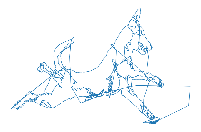
edges_centers_sorted = sort_points(edges_centers)
The image above shows the same points of the previous image, but with sorted points.
The equation in (1) returns complex values whereas the edge signal that I'm intered in is a real 2D function. In this case the Fourier Series representation can be rewritten as: